Note
Click here to download the full example code
Train, convert and predict with ONNX Runtime
This example demonstrates an end to end scenario starting with the training of a machine learned model to its use in its converted from.
Train a logistic regression
The first step consists in retrieving the iris datset.
from sklearn.datasets import load_iris
iris = load_iris()
X, y = iris.data, iris.target

from sklearn.model_selection import train_test_split
X_train, X_test, y_train, y_test = train_test_split(X, y)
Then we fit a model.
from sklearn.linear_model import LogisticRegression
clr = LogisticRegression()
clr.fit(X_train, y_train)
Out:
/opt/miniconda/lib/python3.7/site-packages/sklearn/linear_model/_logistic.py:765: ConvergenceWarning: lbfgs failed to converge (status=1):
STOP: TOTAL NO. of ITERATIONS REACHED LIMIT.

Increase the number of iterations (max_iter) or scale the data as shown in:
    https://scikit-learn.org/stable/modules/preprocessing.html
Please also refer to the documentation for alternative solver options:
    https://scikit-learn.org/stable/modules/linear_model.html#logistic-regression
  extra_warning_msg=_LOGISTIC_SOLVER_CONVERGENCE_MSG)

LogisticRegression()
We compute the prediction on the test set and we show the confusion matrix.
from sklearn.metrics import confusion_matrix

pred = clr.predict(X_test)
print(confusion_matrix(y_test, pred))
Out:
[[10  0  0]
 [ 0 14  0]
 [ 0  1 13]]
Conversion to ONNX format
We use module sklearn-onnx to convert the model into ONNX format.
from skl2onnx import convert_sklearn
from skl2onnx.common.data_types import FloatTensorType

initial_type = [('float_input', FloatTensorType([None, 4]))]
onx = convert_sklearn(clr, initial_types=initial_type)
with open("logreg_iris.onnx", "wb") as f:
    f.write(onx.SerializeToString())
We load the model with ONNX Runtime and look at its input and output.
import onnxruntime as rt
sess = rt.InferenceSession("logreg_iris.onnx")

print("input name='{}' and shape={}".format(
    sess.get_inputs()[0].name, sess.get_inputs()[0].shape))
print("output name='{}' and shape={}".format(
    sess.get_outputs()[0].name, sess.get_outputs()[0].shape))
Out:
input name='float_input' and shape=[None, 4]
output name='output_label' and shape=[None]
We compute the predictions.
input_name = sess.get_inputs()[0].name
label_name = sess.get_outputs()[0].name

import numpy
pred_onx = sess.run([label_name], {input_name: X_test.astype(numpy.float32)})[0]
print(confusion_matrix(pred, pred_onx))
Out:
[[10  0  0]
 [ 0 15  0]
 [ 0  0 13]]
The prediction are perfectly identical.
Probabilities
Probabilities are needed to compute other relevant metrics such as the ROC Curve. Let’s see how to get them first with scikit-learn.
prob_sklearn = clr.predict_proba(X_test)
print(prob_sklearn[:3])
Out:
[[4.15987711e-03 8.54898335e-01 1.40941788e-01]
 [9.44228260e-01 5.57707615e-02 9.78002823e-07]
 [5.17324282e-02 8.88396143e-01 5.98714288e-02]]
And then with ONNX Runtime. The probabilies appear to be
prob_name = sess.get_outputs()[1].name
prob_rt = sess.run([prob_name], {input_name: X_test.astype(numpy.float32)})[0]

import pprint
pprint.pprint(prob_rt[0:3])
Out:
[{0: 0.0041598789393901825, 1: 0.8548984527587891, 2: 0.14094172418117523},
 {0: 0.9442282915115356, 1: 0.055770788341760635, 2: 9.78002844931325e-07},
 {0: 0.05173242464661598, 1: 0.888396143913269, 2: 0.05987146869301796}]
Let’s benchmark.
from timeit import Timer

def speed(inst, number=10, repeat=20):
    timer = Timer(inst, globals=globals())
    raw = numpy.array(timer.repeat(repeat, number=number))
    ave = raw.sum() / len(raw) / number
    mi, ma = raw.min() / number, raw.max() / number
    print("Average %1.3g min=%1.3g max=%1.3g" % (ave, mi, ma))
    return ave

print("Execution time for clr.predict")
speed("clr.predict(X_test)")

print("Execution time for ONNX Runtime")
speed("sess.run([label_name], {input_name: X_test.astype(numpy.float32)})[0]")
Out:
Execution time for clr.predict
Average 8.56e-05 min=7.72e-05 max=0.000101
Execution time for ONNX Runtime
Average 5.02e-05 min=4.61e-05 max=6.17e-05

5.0215695519000296e-05
Let’s benchmark a scenario similar to what a webservice experiences: the model has to do one prediction at a time as opposed to a batch of prediction.
def loop(X_test, fct, n=None):
    nrow = X_test.shape[0]
    if n is None:
        n = nrow
    for i in range(0, n):
        im = i % nrow
        fct(X_test[im: im+1])

print("Execution time for clr.predict")
speed("loop(X_test, clr.predict, 100)")

def sess_predict(x):
    return sess.run([label_name], {input_name: x.astype(numpy.float32)})[0]

print("Execution time for sess_predict")
speed("loop(X_test, sess_predict, 100)")
Out:
Execution time for clr.predict
Average 0.00723 min=0.00694 max=0.00837
Execution time for sess_predict
Average 0.00156 min=0.00152 max=0.00166

0.0015644603711552918
Let’s do the same for the probabilities.
print("Execution time for predict_proba")
speed("loop(X_test, clr.predict_proba, 100)")

def sess_predict_proba(x):
    return sess.run([prob_name], {input_name: x.astype(numpy.float32)})[0]

print("Execution time for sess_predict_proba")
speed("loop(X_test, sess_predict_proba, 100)")
Out:
Execution time for predict_proba
Average 0.0108 min=0.0104 max=0.0115
Execution time for sess_predict_proba
Average 0.0017 min=0.00163 max=0.00188

0.0016972313076257703
This second comparison is better as ONNX Runtime, in this experience, computes the label and the probabilities in every case.
Benchmark with RandomForest
We first train and save a model in ONNX format.
from sklearn.ensemble import RandomForestClassifier
rf = RandomForestClassifier()
rf.fit(X_train, y_train)

initial_type = [('float_input', FloatTensorType([1, 4]))]
onx = convert_sklearn(rf, initial_types=initial_type)
with open("rf_iris.onnx", "wb") as f:
    f.write(onx.SerializeToString())
We compare.
sess = rt.InferenceSession("rf_iris.onnx")

def sess_predict_proba_rf(x):
    return sess.run([prob_name], {input_name: x.astype(numpy.float32)})[0]

print("Execution time for predict_proba")
speed("loop(X_test, rf.predict_proba, 100)")

print("Execution time for sess_predict_proba")
speed("loop(X_test, sess_predict_proba_rf, 100)")
Out:
Execution time for predict_proba
Average 1.25 min=1.23 max=1.26
Execution time for sess_predict_proba
Average 0.00274 min=0.00245 max=0.00442

0.0027408220106735826
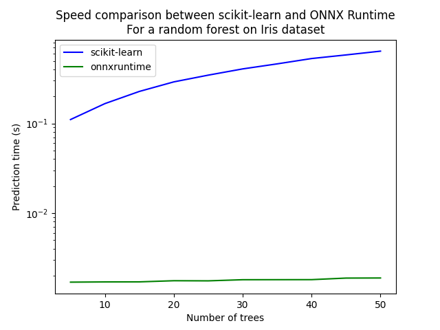
Let’s see with different number of trees.
measures = []

for n_trees in range(5, 51, 5):
    print(n_trees)
    rf = RandomForestClassifier(n_estimators=n_trees)
    rf.fit(X_train, y_train)
    initial_type = [('float_input', FloatTensorType([1, 4]))]
    onx = convert_sklearn(rf, initial_types=initial_type)
    with open("rf_iris_%d.onnx" % n_trees, "wb") as f:
        f.write(onx.SerializeToString())
    sess = rt.InferenceSession("rf_iris_%d.onnx" % n_trees)
    def sess_predict_proba_loop(x):
        return sess.run([prob_name], {input_name: x.astype(numpy.float32)})[0]
    tsk = speed("loop(X_test, rf.predict_proba, 100)", number=5, repeat=5)
    trt = speed("loop(X_test, sess_predict_proba_loop, 100)", number=5, repeat=5)
    measures.append({'n_trees': n_trees, 'sklearn': tsk, 'rt': trt})

from pandas import DataFrame
df = DataFrame(measures)
ax = df.plot(x="n_trees", y="sklearn", label="scikit-learn", c="blue", logy=True)
df.plot(x="n_trees", y="rt", label="onnxruntime",
                ax=ax, c="green", logy=True)
ax.set_xlabel("Number of trees")
ax.set_ylabel("Prediction time (s)")
ax.set_title("Speed comparison between scikit-learn and ONNX Runtime\nFor a random forest on Iris dataset")
ax.legend()
Out:
5
Average 0.11 min=0.107 max=0.118
Average 0.00169 min=0.00161 max=0.00177
10
Average 0.167 min=0.165 max=0.169
Average 0.0017 min=0.00165 max=0.00179
15
Average 0.228 min=0.227 max=0.231
Average 0.0017 min=0.00167 max=0.00172
20
Average 0.291 min=0.286 max=0.296
Average 0.00175 min=0.00173 max=0.00176
25
Average 0.346 min=0.342 max=0.35
Average 0.00174 min=0.00172 max=0.00181
30
Average 0.407 min=0.404 max=0.41
Average 0.0018 min=0.00174 max=0.0019
35
Average 0.463 min=0.459 max=0.467
Average 0.0018 min=0.00176 max=0.00187
40
Average 0.531 min=0.521 max=0.556
Average 0.0018 min=0.00179 max=0.00183
45
Average 0.582 min=0.577 max=0.597
Average 0.00187 min=0.00185 max=0.00189
50
Average 0.642 min=0.64 max=0.645
Average 0.00188 min=0.00185 max=0.00196

<matplotlib.legend.Legend object at 0x7fca300dcda0>
Total running time of the script: ( 5 minutes 52.417 seconds)